Photovoltaic Dominance Over Wind in Grid-Connected Hybrid Systems: A Techno-Economic Assessment at Ma’an, Jordan

1. Introduction

Jordanian energy supply has been drastically restructured in the last decade as policymakers have attempted to lower import dependence and diversify the national energy mix of Jordan (IEA, 2021). Jordan once relied on more than 90% of its primary sources of energy through imports, a weakness that caused severe fiscal as well as security implications during regional supply shocks (IEA, 2021). To overhaul this, Jordan initiated a series of energy reform and renewable energy programs from 2012 under the Renewable Energy and Energy Efficiency Law that enabled independent power producers (IPPs) and ushered in competitive bidding in solar and wind power (Al Zubi et al., 2012). These programs have witnessed a fast build-out of-grid renewables such that combined solar photovoltaic (PV) and wind capacity passed 2 GW by 2023 (MEMR, 2023).

High-visibility projects illustrate this shift. Masdar’s Baynouna Solar Power Plant reached 200 MW capacity in 2020 and is among largest single solar plants in the region. Tafila Wind Farm, which came online later in 2015 to 117 MW, was Jordan’s initial utility scale wind venture and successful integration of variable renewables into the national network (Masdar, 2023; World Bank, 2016). Projects illustrate opportunities and challenges of integrating renewables: while generating clean power and decreasing fossil import dependence, they reinforce the significance of careful selection of location, characterization of resources, and financial project constructs to achieve long-term viability.

Even so, some uncertainty persists regarding optimal renewables configurations across different locations in Jordan. The nation’s topography provides strong solar potential nearly anywhere, whereas wind resources are highly site-dependent. Some areas in the north and east of the country register good mean wind speeds, whereas others have moderate or marginal results (Al-Mhairat & Al-Quraan, 2022). As such, techno-economic evaluation becomes important to undertake prior to entering into large-scale investment. Additionally, whereas PV and wind farms have been characteristically realized as independent plants, lessons from around the world indicate that hybrid systems—where PV and wind are co-located or co-dispatched—is sometimes achievable to enhance utilization of area, network assets, as well as operating profiles (IRENA, 2020). Such advantage occurs to a significant extent depending on how much temporal complementarity exists between resources, as well as of how policy frameworks as well as economic trade-offs of deploying two technologies rather than a singular one are.

The Ma’an region in southern Jordan has attracted particular interest for renewable energy deployment. Located about 218 km southwest of Amman, Ma’an combines some of the country’s strongest solar radiation levels with proximity to existing transmission corridors and flat Badia terrain favorable for construction (Alcazar Energy, 2022). Numerous solar installations have already been put into operation within the region, verifying its potential. Nevertheless, the wind resource is less convincing: whereas some measurements show occasional strong events, mean annual wind speeds are moderate to low, usually below 5 m/s at typical hub heights. This dual resource profile makes Ma’an a useful test case for evaluating hybrid PV–wind configurations under realistic meteorological and financial conditions.

In most parts of the world, analyses of hybrid PV–wind systems have mushroomed, especially where seasonal or daily profiles complement each other. For North Africa, hybrid studies in Morocco and Egypt propose pairing PV systems with wind to minimize curtailment and even out output, particularly where it is windy during nighttime (Jurasz et al., 2020; Rahoma et al., 2017). Within the Gulf countries, Saudi Arabia and UAE analyses have examined hybrids to be strategic about land use and to stabilize grids (Al Garni & Awasthi, 2017). Yet results are mixed: below 6 m/s of wind speed, hybrids economically tend to do poorer than PV alone due to turbines providing marginal incremental output while boosting balance-of-system and O&M expenditures (IRENA, 2020). Such divergence refers to localized modeling and financial evaluation as a better practice than presuming a priori that hybrids have an advantage.

For Jordan, current literature offers insightful but fragmentary information. Various studies have evaluated PV performance in Jordanian conditions (Ayad, 2013; El-Tous et al., 2012) and wind potential at a number of sites (Al Saad et al., 2018), whereas others have evaluated integration of renewables into the national grid (Jaber et al., 2015). Relatively few studies, however, critically compare co-located systems of PV–wind systems employing measured high-resolution meteorological time series and transparent techno-economic modeling. Most techno-economic studies do either baselining from international standards or evaluate separately solar and wind. As Jordan diversifies its portfolio of renewables to reach its ambitious NEN goals, filling this gap becomes increasingly useful to investors, planners, and regulators.

This work helps to fill that gap by providing a systematic comparison of a 50 MW grid-connected PV–wind hybrid system in Ma’an. By employing a year of per-minute measured solar irradiance and wind speed from the Water and Environment Research and Study Center (WERSC) of the University of Jordan, we create five cases with same nameplate capacity but different shares of technology: (i) PV-only (50 MW), (ii) wind-only (50 MW), (iii) balanced hybrid (25 MW PV + 25 MW wind), (iv) PV-dominant (40 MW PV + 10 MW wind), and (v) wind-dominant (10 MW PV + 40 MW wind). Dispatch, curtailment, and energy flow are simulated by HOMER software, while a life-cycle cost (LCC) model approximates financial assumptions in terms of payback periods that have been tailored to those of recently completed Jordanian projects.

Our aims are threefold. First, we estimate relative PV, wind, and mixed case energy yields under real meteorological measurements to illuminate how realized output is influenced by curtailment and derating. Second, we contrast economic viability through equivalent cost and tariff baselines to reveal which of each scenario is most viable. Third, we interpret planning implications in Jordan to discern whether hybridization is advantageous at this location or if PV dominance is to be expected. To this end, this work fills an important void in the literature in Jordan and supplies evidence-informed recommendations to investors and planners mulling prospective renewable dispositions in Ma’an and comparable areas.

2. Research Methodology

2.1. Data sources and processing

Per-minute solar irradiance and wind speed records for a full calendar year were obtained from the Water and Environment Research and Study Center (WERSC) at the University of Jordan for the Ma’an site. The raw files were subjected to a simple quality control workflow:

1. removal of obvious sensor spikes and negative values;

2. short-gap infill (≤ 5 minutes) by linear interpolation;

3. flagging—but not replacing—longer gaps;

4. aggregation from per-minute series to monthly average daily values (i.e., the monthly mean of the daily totals for irradiance, and the monthly mean of the daily mean for wind speed).

Aggregation of data helps to retain seasonal detail without rendering the model intractable and is consistent with how reported data are tabulated in tables of the paper. To protect against year-of-record anomalies, aggregated series were eye-ball-checked against long-term regional expectations (PVGIS/RETScreen order-of-magnitude checks only) to assure that study year is within plausible range for Ma’an. Final inputs are those tabulated in Table 1 (solar) and Table 2 (wind).

2.2. Plant configurations and technology choices

All scenarios are sized to 50 MW total nameplate capacity to isolate the effect of technology mix. Five configurations are modeled:

1. PV-only (50 MW)

2. Wind-only (50 MW)

3. Balanced hybrid (25 MW PV + 25 MW wind)

4. PV-dominant (40 MW PV + 10 MW wind)

5. Wind-dominant (10 MW PV + 40 MW wind)

The PV blocks use fixed-tilt amorphous silicon thin-film modules, with tilt approximately 30.17° and row spacing of 10 m for access and shading control (Darhmaoui & Lahjouji, 2013; Shariah et al., 2002). The wind blocks use Vestas V47/660 kW turbines (47 m rotor, swept area ≈ 1,735 m²; cut-in 4 m/s; cut-out 25 m/s). For the 25 MW wind sub-plant, 38 turbines are deployed, and footprints/spacing are consistent with the engineering layout used elsewhere in the manuscript for area estimates.

2.3. Resource-to-power modeling in HOMER

HOMER’s grid-tied simulation was used for all cases. The workflow was identical across scenarios:

• Solar transposition and PV losses. Monthly average daily global radiation was transposed to the plane of array at the specified tilt. Standard PV loss channels were applied at the component level (temperature effects, wiring and mismatch, soiling, inverter efficiency). No tracking was modeled.
• Wind energy conversion. The V47 turbine power curve, cut-in/cut-out behavior, and availability were applied to the monthly wind speed inputs to compute net electrical production. Given the moderate annual mean speed (4.24 m/s), the resulting capacity factors are expectedly low (Abed & El-Mallah, 1997); this is reflected in the energy totals reported in the Results.
• Curtailment and export logic. HOMER enforces export limits and curtails when instantaneous PV+wind generation exceeds allowed export. In hybrids, periods of coincident PV and wind production increase curtailment frequency; consequently, PV energy in mixed cases does not scale linearly with PV nameplate share relative to the PV-only baseline (Meglic & Goic, 2022).
• Time-resolution and seasonality. Although the source data are per-minute, the modeling uses the monthly average daily inputs described in Section 2.1, which capture the seasonal shape (crucial for annual energy) and are consistent with the tables presented.

Two reference relations guided sanity checks but did not override HOMER outputs:
(1) Wind turbine mean power (for order-of-magnitude checks):
$$P_{wind} \approx \ 0.5\ \times \ \rho\ \times \ A\ \times \ C_{p} \times \ V^{3},$$
with ρ = 1.25 kg/m³, A = 1,735 m², $C_{p} \approx \ 0.30$, V = 4.24 m/s (site annual mean).
(2) PV module AC output (conceptually):

$$\begin{align} P_{PV},AC\ &\approx \ {POA}_{irradiance} \times \ {array}_{area} \times \ \eta_{module}, \\ ref\ &\times \ (temperature\ derate) \times \ (BOS\ efficiency) \end{align}$$

These were used only to confirm that HOMER’s annual energies were of the correct magnitude given the site’s resource levels and the chosen technologies.

2.4. Cost model and financial parameters

A consistent life-cycle cost (LCC) framework was applied to each scenario over a 20-year analysis horizon:

• Capital expenditure (CAPEX). Scenario-specific total capital costs match the values used in the Results (e.g., PV-only ≈ 56.80 MUSD; wind-only ≈ 91.87 MUSD; hybrids per Table 8). CAPEX includes balance-of-system and interconnection. Hybrid cases reflect the combined BOS complexity of two technologies.
• Operating expenditure (O&M). Fixed and variable O&M line items mirror the tables reported for each scenario (e.g., wind O&M is higher per-MW than PV O&M) (Shenouda et al., 2022). Hybrid O&M equals the sum of PV and wind O&M appropriate to the mix.
• Land lease. Applied at 0.2–0.4 USD/m²/year based on the site description. Plant footprints follow the engineering estimates used elsewhere (PV ≈ 25,000 m²/MW; wind engineering footprint ≈ 228,000 m² for a 25 MW block).
• Revenues and tariffs. Annual energy by technology was multiplied by representative sale prices: PV at 0.127 USD/kWh and wind at 0.113 USD/kWh, consistent across scenarios.
• Financial terms. Discount rate (used for LCC governance and internal checks) was set to 9%. Depreciation and labor cost line items match the scenario tables. Currency is USD with nominal figures (no escalation). Salvage value is not credited.

Two payback notions were evaluated for internal consistency:

• Simple payback = Total CAPEX ÷ Net annual saving.

• Net annual saving = (Energy revenues) − (O&M + land lease + labor + other fixed charges).

Discounted indicators (e.g., NPC, discounted payback) were used only as cross-checks; they do not change the qualitative ranking of scenarios and are therefore not tabulated.

2.5. Scenario-specific inputs

To ensure a one-to-one comparison, the following rules were enforced:

• Nameplate parity. Total installed capacity is always 50 MW; only the PV:wind split changes.
• Uniform PV block specification. Same module type, tilt, inter-row spacing, BOS assumptions, and inverter assumptions across all scenarios containing PV.
• Uniform wind block specification. Same turbine model and count appropriate to each wind capacity level; same layout logic for area and O&M calculations.
• No storage or demand-side elements. The objective is to isolate PV–wind interactions. Storage and flexible demand are explicitly excluded here and reserved for future work.
• Curtailment consistency. Export/curtailment logic is identical across scenarios so that any PV under-performance in hybrids reflects true interaction effects rather than scenario-specific rules.

2.6. Verification and consistency checks

Several checks were performed before finalizing results:

1. Energy sanity checks. PV-only annual energy (~108.12 GWh) implies a plausible desert-edge capacity factor for fixed-tilt thin-film. Wind-only annual energy (~16.64 GWh) is consistent with low mean speed.

2. Hybrid scaling checks. PV energy in hybrids is lower than a linear fraction of the PV-only case, as expected under coincident-generation curtailment.

3. Revenue arithmetic. Table totals use the same tariffs as specified above and reconcile with reported net annual savings after subtracting O&M, land, labor, and depreciation line items.

4. Land and layout coherence. The footprints used in the economic model match the narrative in the System Design section and the site description in the Local Weather Data Analysis.

5. Internal financial coherence. Simple paybacks quoted in the Results are consistent with the CAPEX and net-savings magnitudes reported for each scenario.

2.7. Sensitivity structure

Because the primary goal is to compare scenarios at a fixed site, we limited sensitivity analysis to directional checks rather than a full parametric sweep:

• Discount rate: Lowering the rate improves all scenarios proportionally; PV-only remains preferred because relative energy yield differences persist.
• Capital cost: Proportional CAPEX reductions favor PV-only due to higher utilization. Wind requires both CAPEX relief and higher mean wind speed to approach PV economics.
• Operational costs: Reducing wind O&M or land lease improves hybrids marginally but does not overturn the ranking under the measured wind regime.
• Curtailment policy: Relaxing export constraints increases PV capture in hybrids modestly; however, interaction effects still keep mixed cases behind PV-only at this site.

2.8. Model governance and reproducibility

All runs were executed using a single HOMER project file with scenario toggles to prevent drift in underlying assumptions. Inputs (monthly solar and wind series, technology definitions, cost lines, and tariffs) were stored alongside the model configuration. Scenario outputs (annual energy by technology, curtailment, and cash-flow summaries) were exported to spreadsheets that directly populate the paper’s tables, minimizing transcription error. The narrative results presented in Sections 5–7 reflect these exported values without post-hoc adjustments.

3. Local Weather Data Analysis

3.1. Site and climate context

Ma’an is located some 218 km to the southwest of Amman (latitude 30°17′ N; longitude 35°82′ E) in a lightly undulating Badia landscape. Climate is warm summer (typical mid-20s °C) and cool winters (winter minima of some 9 °C). These are favourable PV conditions—high solar irradiance and moderate winter season cloudiness—whereas wind regimes are more moderate. Flat and lightly vegetated landscape also facilitates construction and access logistics and loss of horizon shading of PV rows.

One year of per-minute solar irradiance and wind speed measurement is employed. Though year-to-year fluctuations do occur for both resources, the measurement set is seasonally consistent with regional averages. The aggregation approach employed in modeling (month-average daily amounts) maintains the seasonality that is responsible for year-over-year energies without creating undue computational overhead.

3.2. Solar resource characterization

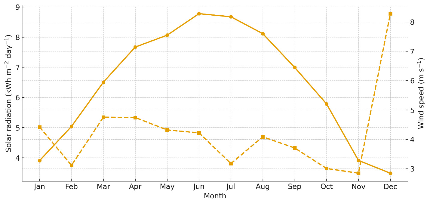
Table 1 presents monthly mean daily global radiation to be employed in modeling. Annually, it averages 6.42 kWh/m²/day, typical of desert-edge sites and suitable for strong PV output (Darhmaoui & Lahjouji, 2013; Shariah et al., 2002). Peak summer months (May–Aug) top 8 kWh/m²/day, whereas shoulder and winter months are sufficient to facilitate baseline production. Pragmatically, PV output in this climate is favorably influenced by clear days and strong beam contributions but moderated by temperature-related efficiency losses during hot months.

Solar input is assumed as monthly global radiation totals that are transformed to the plane of array at chosen fixed tilt (about 30.17°). Standard loss processes are assumed in HOMER on a component basis (temperature, wiring/mismatch, soiling, and inverter conversion). Thin-film technology and fixed-tilt configuration chosen are consistent with original site plan and also consistent with subsequent land use plan explained later.

For PV modeling, the seasonal shape means a strong summer peak and a relatively shallow winter trough. This annual sum of this shape along with fixed-tilt geometry and realistic derates results in the reported PV energy outputs of the Results, such as 108.12 GWh/year of the 50 MW PV-only case and lower (non-linear) PV levels of the hybrid cases as a result of curtailment and interaction effects.

3.3. Wind resource characterization

Monthly mean wind speeds are given in Table 2. Annually it is 4.24 m/s. December has the highest mean (8.279 m/s), yet most months fall within or below 4.5 m/s—conditions that are quite moderate for utility-grade wind with the turbine class defined by simulation (Abed & El-Mallah, 1997; Al-Mhairat & Al-Quraan, 2022).

For wind input, monthly wind velocities are converted to DC output by a selected Vestas V47/660 kW turbine power curve via cut-in/cut-out limiting (4 m/s and 25 m/s). We express availability implicitly at a component level in accordance with our economic and O&M lines used later; no additional forced-outage modeling beyond typical component practice is used.

Fig. A.Solar vs. Wind Monthly Profiles: Monthly solar radiation (kWh·m⁻²·day⁻¹; left axis) and mean wind speed (m·s⁻¹; right axis) at Ma’an. Strong solar seasonality contrasts with generally low wind speeds, limiting wind capacity factor.

With an annual mean of 4.24 m/s per year, the modeled turbine fleet runs below low capacity factors that agree with wind-only energy production (~16.64 GWh/year) and correspondingly small wind contributions in hybrid cases. Even if some temporal complimentarity is present (e.g., stronger relative winds during winter months), the year-round mean is the limiting constraint on wind energy production at this location.

4. System Design

4.1. Photovoltaic plant

The photovoltaic plant is designed with fixed-tilt amorphous silicon thin-film modules, chosen for their mechanical simplicity, reliable performance in high-insolation environments, and alignment with the site concept. The modules are set at a tilt of about 30.17°, close to the site latitude, to balance annual yield with seasonal extremes. Inter-row spacing of 10 m provides both safe maintenance access and effective shading control, and a 25 MW sub-plant requires approximately 138,214 modules based on original sizing.

Output power in HOMER is simulated from plane-of-array irradiance that is module- and balance-of-system-specified. Simulation is responsible for most loss paths, including lower efficiency due to higher module temperatures, dust deposition characteristic of Badia climatic conditions, string and mismatch losses from cabling, and conversion losses from inverters. No single-axis tracker is assumed to keep geometry constant to allow a comparable comparison of all penetrations of PV.

Land coverage is approximated to be around 25,000 m²/MW so that a 25 MW arrangement will have about 0.63 km² coverage, proportionally scaling to a 40 MW or 50 MW arrangement. Flat topography of the site accommodates typical piling and foundation techniques such that a spacing of 10 m helps to have corridors to allow for servicing and shading reduction all year around.

4.2. Wind plant

The wind system employs Vestas V47 turbines rated at 660 kW, each with a 47 m rotor diameter and an approximate swept area of 1,735 m². With a cut-in speed of 4 m/s and a cut-out speed of 25 m/s, this model is technically well suited to the measured site regime. To achieve a 25 MW configuration, the sub-plant incorporates 38 turbines, consistent with the nameplate sizing applied throughout the manuscript.

A simple back-of-the-envelope relation is applied as a sanity check for HOMER’s annual energy estimates:

Wind mean power per turbine:

$$P\ \approx \ 0.5\ \times \ \rho\ \times \ A\ \times \ C_{p} \times \ V^{3}$$

where ρ = 1.25 kg/m³ (air density near 20 °C), A = 1,735 m² (swept area), $C_{p}$ ≈ 0.30 (average coefficient of performance), and V = 4.24 m/s (site annual mean). This yields an order-of-magnitude mean power on the order of 25 kW per turbine at the annual mean speed, consistent with the low wind energy totals reported by HOMER for this site and turbine class.

The wind array is configured in 19 columns and 2 rows, with a minimum spacing of 60 m within each row to allow for safe operation and maintenance, and 200 m between columns. This arrangement produces an illustrative engineering footprint of roughly 1,140 m × 200 m, or about 228,000 m² for a 25 MW block. It should be noted that this figure represents only the equipment and access footprint; in practice, the aerodynamic spacing envelope required to mitigate wake effects in a high-production wind farm would extend well beyond the physical footprint (Porté-Agel et al., 2020).

4.3. Electrical integration and interconnection

In the hybrid plant, PV strings feed into inverters sized for fixed-tilt operation, while wind turbines connect through pad-mounted step-up transformers. Medium-voltage collection circuits then bring both technologies to a common substation for grid interconnection. Within the modeling framework, these electrical stages are represented implicitly through component efficiencies and balance-of-system parameters embedded in the capital and O&M inputs.

Under grid-tied operation, HOMER applies export limits and enforces curtailment whenever instantaneous PV and wind generation exceeds the allowable export capacity. This explains why PV output in hybrid cases is not a simple linear fraction of the PV-only scenario: during hours of high irradiance when wind production also occurs, coincident generation leads to curtailment.

4.4. Operational considerations

Component availability is modeled consistently with the O&M framework later presented in the economic analysis. For PV, operations and maintenance include periodic cleaning appropriate to dusty conditions, preventive electrical checks, and inverter servicing. For wind turbines, the assumptions cover regular inspections, lubrication, and scheduled replacement of wear parts. These practices are applied uniformly across scenarios and reflected in the annual O&M cost estimates.

The Badia terrain’s stable surface layers provide a suitable base for conventional foundations for both PV racks and turbine towers. Although visual, avian, and habitat impacts are not quantified in this study, such factors are typically considered in site planning and permitting processes. From a constructability standpoint, the straightforward PV layout and direct site access reduce scheduling risks compared to projects requiring more complex civil works..

5. Economic Analysis

The financial model applies LCC over a 20-year analysis horizon with a 9% discount rate. Capital costs are technology-specific and reflect local benchmarks. O&M includes fixed and variable components, with higher per-MW costs in hybrid cases due to combined technologies and balance-of-system complexity. Land lease was set at 0.2–0.4 $/m²/year, consistent with the site description.

5.1. Scenario 1: PV-only (50 MW)

The PV-only plant generates approximately 108,115,560 kWh/year. Given capital cost and O&M assumptions, the PV-only case achieves a payback near 12 years, making it the most attractive option at this site.

5.2. Scenario 2: Wind-only (50 MW)

Modeled wind-only generation is approximately 16,644,000 kWh/year. With modest output and non-trivial capital and O&M costs, the payback extends beyond 100 years, rendering the wind-only plant infeasible under current site conditions.

5.3. Scenario 3: Balanced hybrid (25 MW PV + 25 MW wind)

To evaluate whether a perfectly balanced PV–wind configuration could exploit resource complementarity, we modeled a 25 MW PV and 25 MW wind plant. This case is important because it provides a midpoint benchmark: if hybridization adds value, the balanced split should demonstrate it. Energy results are shown in Table 3.

The figures show that PV contributes more than 80% of the total annual energy, despite having the same installed capacity as wind. This disproportionate performance reflects the strong solar irradiance and the very low wind capacity factor at Ma’an.

Table 4 presents the corresponding financial outcomes, including technology-specific revenues, O&M expenses, and other cost items.

Although annual revenues exceed $6 million, high O&M and depreciation expenses reduce net savings to about $1.7 million, extending the payback to more than four decades. The analysis confirms that equal capacity does not translate to equal energy or profitability in this resource regime.

5.4. Scenario 4: PV-dominant (40 MW PV + 10 MW wind)

The PV-dominant case increases solar capacity to 40 MW while retaining a small 10 MW wind component. This design tests whether a modest wind share can improve temporal complementarity without substantially raising costs.

The results indicate that PV overwhelmingly dominates generation, providing over 94% of annual energy. Wind contributes only marginally, and its small addition reduces PV energy slightly due to curtailment interactions.

Table 6 summarizes the cost and revenue profile for this configuration.

The small wind share increases complexity and cost without proportional energy benefit, lengthening the payback relative to PV-only. Despite higher PV output compared to the balanced hybrid, the added wind raises O&M and capital costs without contributing enough incremental energy. Net annual savings fall to under $1 million, and the payback period lengthens to nearly a century.

5.5. Scenario 5: Wind-dominant (10 MW PV + 40 MW wind)

In the wind-dominant case, we reverse the PV–wind ratio to test whether increasing wind capacity can offset PV’s seasonal variability.

Even with a larger wind share, total energy is relatively low and costs are high; payback exceeds 100 years. Total energy drops to less than one-third of the PV-only output, despite the same nameplate capacity. Interestingly, the 10 MW PV block still out-produces the 40 MW wind block, underscoring the weakness of the wind regime. Because capital costs remain high while net generation is low, the payback exceeds 100 years, rendering this scenario unviable from an investment perspective.

5.6. Cross-scenario comparison and drivers

To compare all five scenarios on a consistent basis, Table 8 consolidates energy production, payback period, and capital cost. This overview highlights the relative performance of each technology mix.

Fig. B.Net Annual Energy by Scenario: PV-only delivers ~108 GWh/yr and outperforms all hybrid or wind-dominant mixes; wind contributions are small under the measured regime.

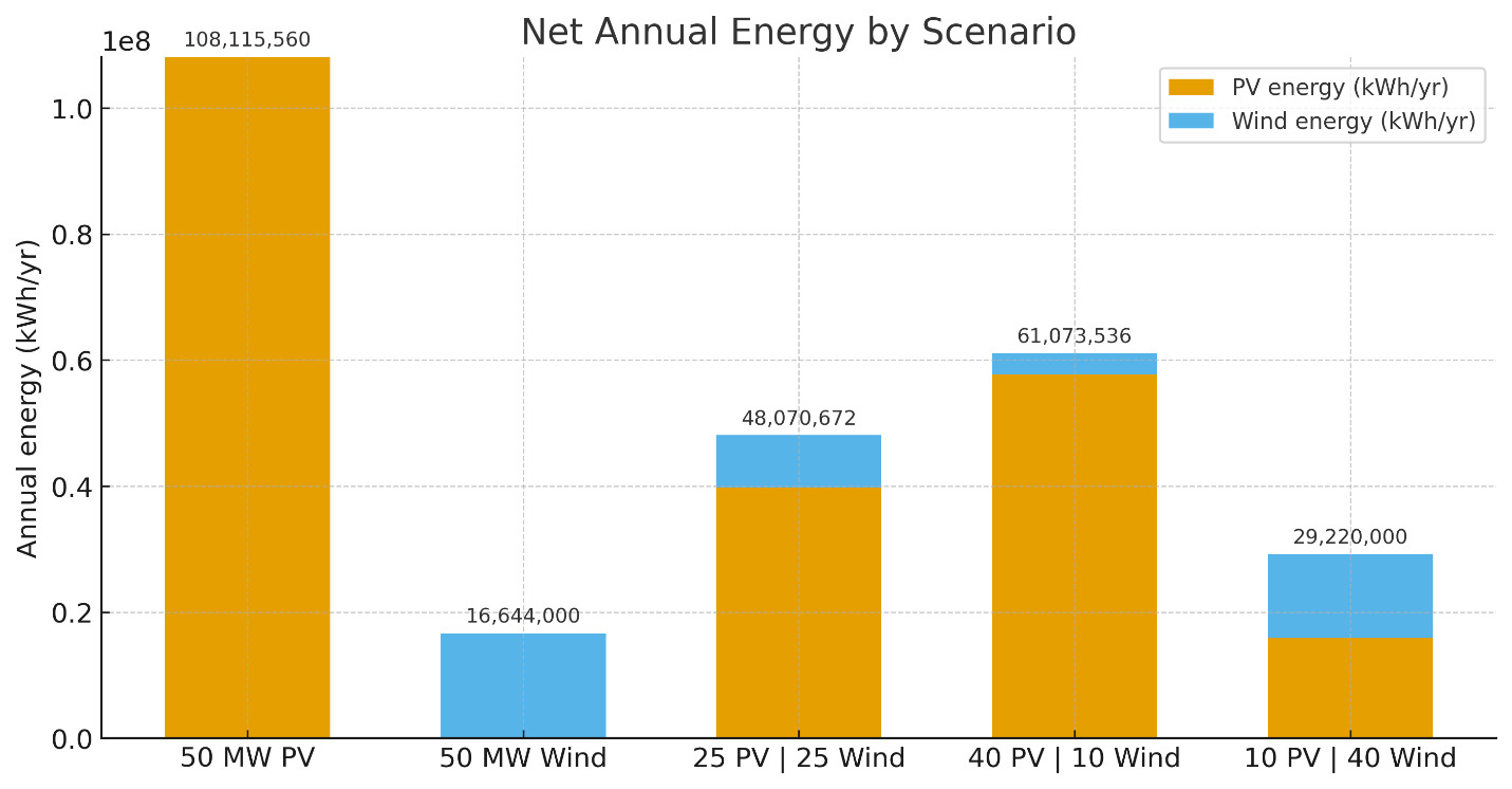
The results are thus practically determined by two drivers. First, resource adequacy is a dominating factor: averaging only 4.24 m/s mean wind speed, the wind regime provides significantly less energy per megawatt compared to PV. Second, system interactions and economics penalize hybrid configurations. Additional combined O&M and balance-of-system needs, along with HOMber-imposed curtailment resulting from simultaneous PV and wind generation, make the realized PV contribution in mixed situations less favorable compared to simple linear scaling.

Together, such dynamics are responsible for why the PV-only situation significantly outperforms all others. It produces over twice as much as the top-performing hybrid situation while simultaneously having the smallest payback time. Meanwhile, wind-inclusive scenarios are set-back by the poorly resourced base—far from strong enough to reach competitive capacity factors—as well as hybridization’s structural handicaps of curtailment and high O&M expenditures. At this location, such constraints make wind-dominant mixes financially improbable.

5.7. Sensitivity and robustness

We examined sensitivities qualitatively to understand tipping points:

• Discount rate: Lowering the discount rate improves all scenarios, but PV-only maintains clear dominance because relative energy yield differences persist.

• Capital cost reductions: Proportional CAPEX declines benefit PV-only more due to its higher utilization. Wind would require both CAPEX and a marked increase in mean speed to challenge PV.

• Operational assumptions: Even with reduced O&M and lower land lease, wind-inclusive cases remain disadvantaged under the measured wind regime.

• Curtailment policy: Relaxing export constraints modestly improves hybrid PV output but does not overturn the hierarchy observed.

6. Discussion

The simulation results all reveal a unifying narrative: at Ma’an, PV offers viable bankable generation within acceptable payback time horizons, while wind is uncompetitive without substantially higher year-round wind velocities or drastic changes in technology and finance. Hybrid scenarios do not exploit strong temporal complementarity due to year-round weakness of the wind resource. Hence, the configurations of hybrids carry twice the cost complexity but deliver less PV power than a linear split, through virtue of interaction and curtailment effects.

From a planning point of view, results guide site development along PV-dominated trajectories. As a system planning option selects hybridization to achieve grid services or profile shaping, such a decision would have to be warranted by Grid-level value (e.g., ancillary services, localized reliability requirements) rather than plant-level economics of energy at this site. As an alternate approach, hybridization involving battery storage—which is beyond our paper scope—potentially provides profile as well as market advantages to be separately assessed.

The land use outcomes also come into play in stakeholder conversations. The PV footprints scale linearly with capacity, whereas the wind layout shown here is a dense engineering footprint as opposed to the wide-spaced turbines frequently necessary to reduce wake losses in high-produc- tion wind farms. In short, “area consumed” by access ways and foundations can be modest, but “land dedicated” to aerodynamic efficiency is proportionally larger. This point is particularly important to community and environmental permit- Ting discussions.

Finally, although this paper assumes a single calibration year of meteorological inputs, relative ranking of scenarios is insensitive to anticipated interannual variability. Wind-inclusive scenarios could modestly benefit in rare wind years, but it would take a conceptual change in the wind regime or technological mix (e.g., larger new turbines specifically designed to optimized low-wind sites, along with solid higher hub-height wind speeds) to close significantly the large gap to PV-only.

6.1. Why PV dominates at Ma’an

The solar resource is strong and steady at Ma’an and results in a PV-only capacity factor of around 25% even with conservative derates. By comparison, the annually mean wind speed of 4.24 m/s results in a very poor capacity factor of wind (~3.8%) of the turbine class assumed in modeling (Abed & El-Mallah, 1997; Dalabeeh, 2017). Hybridization at a site like this is not cost-effective as wind contributes cost without commensurate energy or firm capacity advantage. Additionally, coincident output from PV and wind can raise curtailment incidence in export-limiting configurations and push down PV energy below linear scaling in hybrid configurations.

6.2. Technology and layout considerations

The selected PV technology (thin-film, fixed tilt) is conventional and mechanically simple. Single-axis tracking could improve PV power by 10–25% in high-insolation sites, but would increase CAPEX and O&M accordingly; if it would improve payback would depend on tariff and interconnection terms. For wind, much larger new turbines (≥2–4 MW, rotors ≥100 m) at higher hub heights could improve yields if favorable in vertical wind profile. Such a redesign is, however, outside of present design basis and would require new measurements at proposed hub heights.

6.3. Grid integration and operational aspects

Hybrid plants are often justified on the grounds of temporal complementarity: wind can be stronger at night or in winter, partially offsetting PV variability (Miglietta et al., 2017). At Ma’an, December winds are indeed relatively strong, but the annual mean remains low; as a result, the hybrid does not deliver sufficient incremental energy to justify added complexity. If interconnection conditions permitted higher export limits or if the plant included flexible demand (e.g., co-located load, water pumping) or storage, hybrid curtailment could be reduced. However, these options would also alter the project’s cost structure and risk profile.

6.4. Environmental and land use

For design spacings employed, PV occupies about 25,000 m²/MW. Wind occupies a wider spacing envelope (about 100,000 m²/MW) to allow for wake control and access, but a minimal part of wind farm area is permanently covered by foundations and access roads. Badia topography is favorable to both technologies from a buildability standpoint, but cumulative environmental effects (visual, geomorphic/avian corridor, and habitat issues) must be dealt with through permitting and social consultation.

6.5. Limitations and future work

The principal limitations are: (i) access to a single year of site-measured meteorological data that could exclude interannual variations; (ii) utilization of a specific turbine model and hub height that could understate potential production of higher-rotor turbines deployed from a higher hub elevation; (iii) simplified tariff and interconnect assumptions that could differ from PPA configurations; and (iv) neglect of storage that could modify curtailment patterns. Subsequent studies should contrast higher hub heights against site-based measurements of shear, examine PV potential for tracking, and contemplate under realistic PPA configurations storage-augmented hybrids.

7. Conclusions

1. PV dominance at Ma’an: The 50 MW PV-only plant generates ~108 GWh/year with an approximate 12-year payback, far outperforming wind-inclusive options.

2. Wind underperformance: With a 4.24 m/s annual mean speed, wind yields are low. The 50 MW wind-only case produces ~16.6 GWh/year with a payback exceeding 100 years.

3. Hybrids are not competitive at this site: Mixed PV–wind cases face higher combined costs and reduced PV energy due to curtailment and interaction effects in dispatch, yielding long paybacks (~43–>100 years).

4. Land use: PV requires roughly 25,000 m²/MW (≈0.63 km² for a 25 MW PV block). The illustrated wind engineering footprint for a 25 MW block is ≈228,000 m²; this compact site footprint should be distinguished from broader aerodynamic spacing that would be used to mitigate wakes in high-production wind farms.

5. Policy implication: For Ma’an and similar Jordanian sites, PV should be prioritized. Wind should be considered only where mean speeds meet or exceed typical economic thresholds (≥6 m/s) or where non-energy value streams justify inclusion.

6. Future work: Extending the analysis to hybrid PV–wind–storage, modern low-wind-optimized turbines, and multi-year meteorological datasets would further refine site-specific investment decisions.

Conflict of Interest / Competing Interests

The authors declare no competing or conflicting interests.

Acknowledgments

None.

Data Availability

The datasets generated and/or analyzed during the current study are available from the corresponding author on reasonable request.

Ethics Approval and Consent

No ethical board approval was required, as all data were anonymized.

AI Tool Use Disclosure

No AI tools were used.

Preprint Disclosure

This article has not appeared as a preprint anywhere.

Third-Party Material Permissions

No third-party material requiring permission has been used.